2022-06-15
Protein encodings
Introduction
There are countless examples in the literature where deep learning is used to make predictions using protein sequences. In order to use protein sequences as inputs for deep learning models they need to be transformed into numerical descriptors. This can be performed in several different ways depending on the underlying data and the purpose of the model. In this notebook I highlight four different ways to generate such numerical features from protein sequences using; 1) the Amino Acid composition, 2) generation of N-grams, 3) creation of word embeddings and 4) BLOSUM matrices. To illustrate how to use these descriptors I use them to train a deep learning model to predict protein classifications. The models themselves were kept as basic as possible and although reaching good accuracy were not fully optimized.
Libraries
The below libraries were used to process the data and build the models.
Show code
# import the necessary packages
from collections import Counter
from keras.preprocessing.text import Tokenizer
from keras.preprocessing.sequence import pad_sequences
from sklearn.model_selection import train_test_split, KFold
from sklearn.compose import ColumnTransformer
from sklearn.preprocessing import MinMaxScaler, LabelBinarizer, OneHotEncoder
from sklearn.feature_extraction.text import CountVectorizer
from sklearn.pipeline import Pipeline
from sklearn import preprocessing
from tensorflow.keras.callbacks import EarlyStopping
from tensorflow.keras.models import Model
from tensorflow.keras.models import Sequential
from tensorflow.keras.layers import Dense, Activation, Dropout, Embedding, Flatten, Concatenate, Input, Conv1D, MaxPooling1D, LeakyReLU, LSTM, BatchNormalization
from tensorflow.keras.optimizers import Adam
from keras.losses import mean_squared_error
from sklearn.metrics import r2_score, accuracy_score
from keras import backend as K
from keras.utils.np_utils import to_categorical
from sklearn import linear_model
import matplotlib.pyplot as plt
import pandas as pd
import numpy as np
import cv2
np.random.seed(1337) # for reproducibility
Data
The dataset was compiled form the Protein Data Bank and posted by SHAHIR on kaggle for people to use to test different modeling approaches. The PDB database is used to visualize and store three-dimensional structural data of proteins. Each structure comes with a comprehensive list of all the experimental details that was used to generate the structure and the characteristics of the protein. It also classifies the protein into a family based on structural and sequence similarity with other proteins.
Processing
Before using the data several steps were performed to make it more presentable for our deep learning model which is outlined below.
The data consists of two separate files. One file containing all the details about the structure and a second file containing the details on the protein sequence. Both files are loaded and merged together based on Structure ID. The file also contains structural data from DNA and RNA. These will be removed as we are only interested in the protein structures. We are only interested in the protein IDs and the sequences so we drop all other columns.
pdb_data_no_dups = pd.read_csv("Data/pdb_data_no_dups.csv")
#pdb_data_no_dups = pdb_data_no_dups[[""]]
pdb_data_seq = pd.read_csv("Data/pdb_data_seq.csv")
#Merge data on structureId and select only protein structures
data_merged = pdb_data_no_dups.merge(pdb_data_seq, how='inner', on='structureId').query('macromoleculeType_x == "Protein"')
#Select columns we are interested in and remove duplicates
data_merged = data_merged[["structureId", "classification", "sequence"]]
data_merged = data_merged.drop_duplicates(["structureId", "classification", "sequence"])
data_merged = data_merged.reset_index(drop=True)
#Print data
'The data has {} rows and {} columns'.format(data_merged.shape[0], data_merged.shape[1])
## 'The data has 166681 rows and 3 columns'
pd.set_option('display.max_columns', None)
data_merged
Show code
##        structureId                            classification  \
## 0             101M                          OXYGEN TRANSPORT
## 1             102L                     HYDROLASE(O-GLYCOSYL)
## 2             102M                          OXYGEN TRANSPORT
## 3             103L                     HYDROLASE(O-GLYCOSYL)
## 4             103M                          OXYGEN TRANSPORT
## ...            ...                                       ...
## 166676        9RSA            HYDROLASE (PHOSPHORIC DIESTER)
## 166677        9RUB                      LYASE(CARBON-CARBON)
## 166678        9WGA                       LECTIN (AGGLUTININ)
## 166679        9XIA  ISOMERASE(INTRAMOLECULAR OXIDOREDUCTASE)
## 166680        9XIM  ISOMERASE(INTRAMOLECULAR OXIDOREDUCTASE)
##
##                                                  sequence
## 0       MVLSEGEWQLVLHVWAKVEADVAGHGQDILIRLFKSHPETLEKFDR...
## 1       MNIFEMLRIDEGLRLKIYKDTEGYYTIGIGHLLTKSPSLNAAAKSE...
## 2       MVLSEGEWQLVLHVWAKVEADVAGHGQDILIRLFKSHPETLEKFDR...
## 3       MNIFEMLRIDEGLRLKIYKDTEGYYTIGIGHLLTKSPSLNSLDAAK...
## 4       MVLSEGEWQLVLHVWAKVEADVAGHGQDILIRLFKSHPETLEKFDR...
## ...                                                   ...
## 166676  KETAAAKFERQHMDSSTSAASSSNYCNQMMKSRNLTKDRCKPVNTF...
## 166677  MDQSSRYVNLALKEEDLIAGGEHVLCAYIMKPKAGYGYVATAAHFA...
## 166678  ERCGEQGSNMECPNNLCCSQYGYCGMGGDYCGKGCQNGACWTSKRC...
## 166679  MNYQPTPEDRFTFGLWTVGWQGRDPFGDATRRALDPVESVQRLAEL...
## 166680  SVQATREDKFSFGLWTVGWQARDAFGDATRTALDPVEAVHKLAEIG...
##
## [166681 rows x 3 columns]
Rows with missing values are removed
data_merged.isna().sum()
## structureId       0
## classification    1
## sequence          3
## dtype: int64
data_merged = data_merged.dropna()
Having a closer look at the data one can see that some of the sequences contain AAs other then the 21 standard ones (B|O|U|X|Z).
#Count all different AAs
sequences = data_merged["sequence"].dropna()
charCounter = CountVectorizer(analyzer="char", ngram_range=(1,1))
charVec = charCounter.fit_transform(sequences.to_numpy())
AA = charCounter.get_feature_names_out()
AAcounts = np.asarray(charVec.sum(axis=0))[0]
print(dict(zip(AA, AAcounts)))
## {'a': 3378009, 'b': 19, 'c': 642515, 'd': 2484519, 'e': 2835673, 'f': 1746745, 'g': 3211970, 'h': 1176659, 'i': 2389749, 'k': 2517051, 'l': 3940616, 'm': 1001217, 'n': 1857711, 'o': 2, 'p': 2048893, 'q': 1659623, 'r': 2136127, 's': 2837198, 't': 2460573, 'u': 50, 'v': 2990099, 'w': 628670, 'x': 177570, 'y': 1546907, 'z': 28}
For the sake of simplicity I decided to remove all those sequences.
#Remove sequences that contain non standard AAs
AA_mask = sequences.str.contains('^[RHKDESTNQCGPAILMFWYV]+$')
data_merged = data_merged.loc[AA_mask]
'{} rows were removed'.format((AA_mask == False).sum())
## '4377 rows were removed'
If we look at the size distribution of the sequences we can see that quite a large proportion consists of sequences shorter then 20 AAs.
seqLengths = data_merged["sequence"].str.len()
lengths = Counter(seqLengths.to_list())
plt.clf()
# visualize
_ = plt.hist(seqLengths.to_list(), bins=120, edgecolor='black')
_ = plt.xlim(0, 1200)
plt.show()
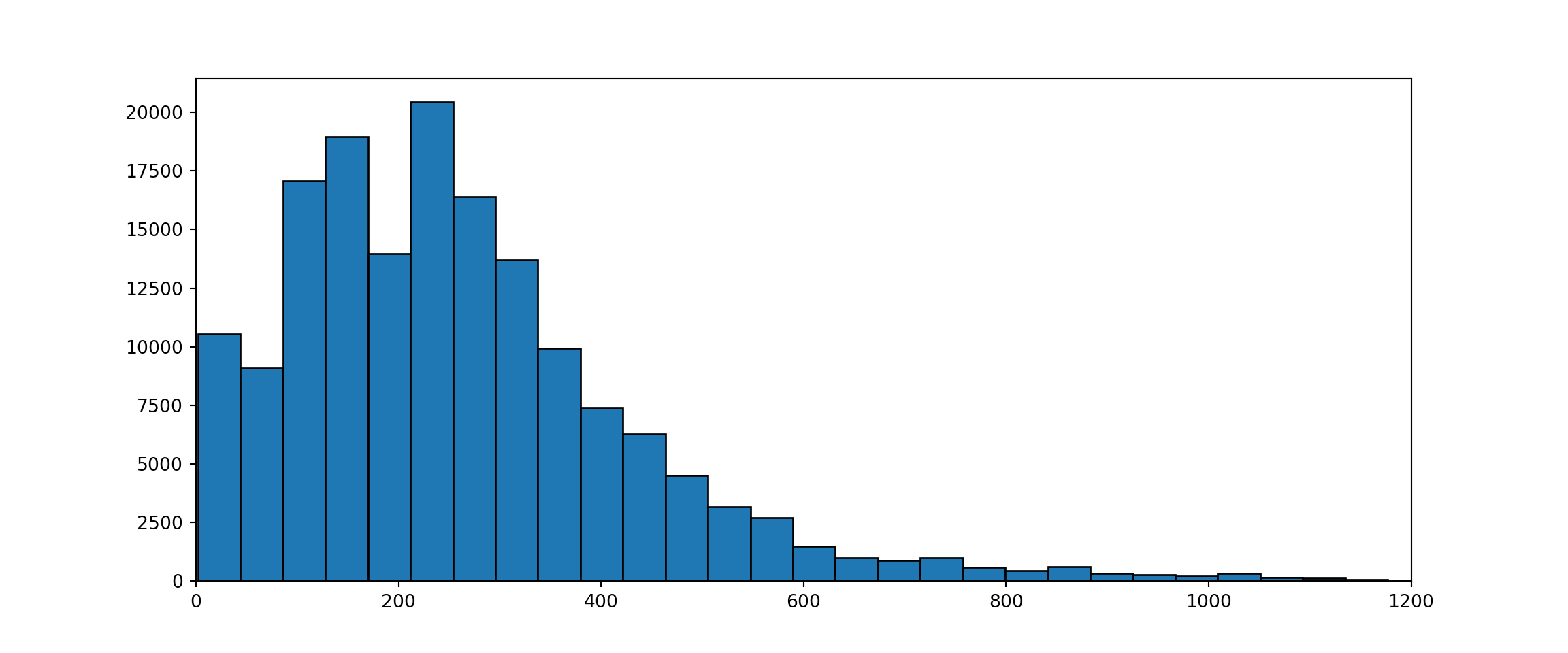
These are most likely from proteins for which only part of the structure has been solved and it will be hard to predict an accurate classification for those. To get more accurate models I removed all sequences that have a length with less then 20 AAs.
#Filter out sequences that are shorter then 20 AAs
AA_length_mask = data_merged["sequence"].str.len() >= 20
data_merged = data_merged.loc[AA_length_mask]
There are >4000 different classifications defined. Most of them consisting of far to little sequences to train a model.
data_merged.groupby(["classification"])["classification"] \
  .count() \
  .sort_values(ascending = False)
Show code
## classification
## HYDROLASE                        23465
## TRANSFERASE                      16557
## OXIDOREDUCTASE                   14288
## IMMUNE SYSTEM                     7920
## HYDROLASE/HYDROLASE INHIBITOR     5661
##                                  ...
## NOVEL SEQUENCE                       1
## NONSTRUCTURAL PROTEIN                1
## NON-HEME IRON PROTEIN                1
## NK CELL                              1
## virus/inhibitor                      1
## Name: classification, Length: 4383, dtype: int64
To build the models I focus on the top 10 classifications.
#Filter for top10 classifications
classes = 10
data_merged['count'] = data_merged.groupby(["classification"])["classification"].transform('count')
top_class = data_merged["count"].sort_values(ascending=False).unique()[classes]
data_top_classes = data_merged[data_merged["count"] > top_class].sort_values(by=["count"], ascending=False)
data_top_classes = data_top_classes.reset_index(drop=True)
#Print results
data_top_classes.groupby(["classification"])["classification"] \
  .count() \
  .sort_values(ascending = False)
Show code
## classification
## HYDROLASE                        23465
## TRANSFERASE                      16557
## OXIDOREDUCTASE                   14288
## IMMUNE SYSTEM                     7920
## HYDROLASE/HYDROLASE INHIBITOR     5661
## LYASE                             4476
## TRANSCRIPTION                     4288
## TRANSPORT PROTEIN                 3751
## SIGNALING PROTEIN                 3284
## VIRAL PROTEIN                     2761
## Name: classification, dtype: int64
Transformation
To build the models we binarize the classes. See: link for an explanation on choosing the right encoding method.
lb = LabelBinarizer()
y = lb.fit_transform(data_top_classes["classification"])
y[1:10]
## array([[1, 0, 0, 0, 0, 0, 0, 0, 0, 0],
##        [1, 0, 0, 0, 0, 0, 0, 0, 0, 0],
##        [1, 0, 0, 0, 0, 0, 0, 0, 0, 0],
##        [1, 0, 0, 0, 0, 0, 0, 0, 0, 0],
##        [1, 0, 0, 0, 0, 0, 0, 0, 0, 0],
##        [1, 0, 0, 0, 0, 0, 0, 0, 0, 0],
##        [1, 0, 0, 0, 0, 0, 0, 0, 0, 0],
##        [1, 0, 0, 0, 0, 0, 0, 0, 0, 0],
##        [1, 0, 0, 0, 0, 0, 0, 0, 0, 0]])
The sequences are transformed to a numpy array.
X = data_top_classes["sequence"].to_numpy()
Amino Acid composition model
As a first most basic model we can use the Amino Acid (AA) composition of each sequence to train our model. To do this we count the number of AAs for each sequence.
vectorizer = CountVectorizer(analyzer="char")
X_vec = vectorizer.fit_transform(X)
X_AAC = X_vec.toarray()
feature_names = vectorizer.get_feature_names_out()
pd.DataFrame(X_AAC, columns = feature_names)
Show code
##         a  c   d   e   f   g   h   i   k   l  m   n   p   q   r   s   t   v  \
## 0      22  1  23  20  11  16   6  27  29  18  2  16  19   7   6  13  19  14
## 1      19  4  20  15   8  18  11  17  18  24  8   9  13   4  11  18  17  10
## 2      23  3  21  23  19  29   7  26  17  23  8  24  22  11  18  31  26  12
## 3      23  3  21  22  19  29   7  26  17  23  8  24  22  12  18  31  26  12
## 4      40  0  22  16   9  26  13  16   9  23  5  11  20  13  15  13  28  28
## ...    .. ..  ..  ..  ..  ..  ..  ..  ..  .. ..  ..  ..  ..  ..  ..  ..  ..
## 86446  13  4   4   3   4  18   0   5   5  11  2   4   6   8   5  16   8   9
## 86447  20  5  12  13  18  25   6  10   7  30  4  21  29  17  12  20  30  22
## 86448  12  2   5   5   5  15   1   2   4   7  3   4   3   8   8  13   9   7
## 86449  16  5  20   9  20  25   7  10   6  28  3  19  28  20  14  22  20  22
## 86450  53  3  28  28  17  32   6  30  35  45  7  28  24  19  13  19  24  25
##
##         w   y
## 0       6  11
## 1       1   9
## 2      11  26
## 3      11  26
## 4       4  12
## ...    ..  ..
## 86446   2   8
## 86447   5   9
## 86448   3   8
## 86449   4  10
## 86450  10  17
##
## [86451 rows x 20 columns]
AAC Model
For the AA model I use three dense layers with the last layer having 10 units which is equal to the amount of classes that we try to predict. I use early stopping based on the accuracy of the test data to avoid over fitting. To limit the training time I increased the batch size to 128. The model is wrapped into a function such that I can re-use the model for Cross Validation.
Show code
def Model_AAC(X_train, y_train, X_test, y_test, classes = 10):
    #Define model
    model = Sequential()
    model.add(Dense(16, input_dim=X_train.shape[1], activation="relu"))
    model.add(Dense(8, activation="relu"))
    model.add(Dense(classes, activation="softmax"))
    #Define optimizer
    opt = Adam(learning_rate=0.01)

    early_stopping = EarlyStopping(min_delta=0.01,
                                   patience=5,
                                   monitor='val_accuracy',
                                   verbose=0,
                                   mode="max",
                                   restore_best_weights=True
                                   )
    #Compile model
    model.compile(loss='categorical_crossentropy', optimizer=opt, metrics=['accuracy'])

    model.fit(x=X_train, y=y_train,
              validation_data=(X_test, y_test),
              epochs=100,
              callbacks=[early_stopping],
              verbose=0,
              batch_size=128)

    y_pred = model.predict(X_test)
    test_acc = accuracy_score(np.argmax(y_test, axis=1), np.argmax(y_pred, axis=1))
    return test_acc
Valdidation
To test the model we check its performance on the test data that we set apart and using 5-fold cross validation.
Training data
To asses the model the data is split into a train set and 20% of the data is held back to evaluate our model. To avoid bias I normalized the data using the MinMaxScaler() (see: link for an explanation on normalization of data).
#Generate train and test data
X_train, X_test, y_train, y_test = train_test_split(X_AAC, y, test_size=.2, random_state=42, shuffle=True)
#Scale data
scaler = MinMaxScaler()
X_train = scaler.fit_transform(pd.DataFrame(X_train, columns = feature_names)) #Fit and transform data on training data
X_test = scaler.transform(pd.DataFrame(X_test, columns = feature_names)) #Transform data using the training parameters for fitting.
#Fit data to Model
train_acc = Model_AAC(X_train, y_train, X_test, y_test)
print("Accuracy-train = {:.3f}".format(train_acc))
## Accuracy-train = 0.452
Cross Validation
Estimate accuracy using 5-fold cross validation.
Show code
#Generate X, y data
ACC = []
kf = KFold(n_splits=5, random_state=42, shuffle=True)
i = 1
for train_index, test_index in kf.split(X_AAC):
    X_train, X_test = X_AAC[train_index], X_AAC[test_index]
    y_train, y_test = y[train_index], y[test_index]

    scaler = MinMaxScaler()
    X_train = scaler.fit_transform(pd.DataFrame(X_train))
    X_test = scaler.transform(pd.DataFrame(X_test))

    pred = Model_AAC(X_train, y_train, X_test, y_test)
    print("Accuracy-fold-{} = {:.3f}".format(i, pred))
    i = i+1

    ACC += [pred]
## Accuracy-fold-1 = 0.435
## Accuracy-fold-2 = 0.448
## Accuracy-fold-3 = 0.428
## Accuracy-fold-4 = 0.443
## Accuracy-fold-5 = 0.429
print("Accuracy-mean = {:.3f}".format(np.mean(ACC, dtype=object)))
## Accuracy-mean = 0.437
Conclusion
Using the AA composition alone we get an accuracy of around 0.4. This is not too bad considering we are trying to predict 10 different classes. This type of encoding can work well for shorter sequences like peptides. However, with this type of encoding any information on the order of the sequences is lost. Especially for longer sequences this is important as many classes are defined by specific domains within the sequence.
N-grams model
To preserve some information on the order of AAs in the sequences we can count the occurrences of the most common AA combinations across all the sequences. In the below example we look at the 20 most common 3 letter AA combinations and then count the occurrence of each for all the sequences.
vectorizer = CountVectorizer(analyzer="char", ngram_range=(3,3), max_features = 20)
X_train_vec = vectorizer.fit_transform(X)
feature_names = vectorizer.get_feature_names_out()
#Print results
pd.DataFrame(X_train_vec.toarray(), columns = feature_names)
Show code
##        aaa  aag  aal  ala  ale  all  avl  eal  ell  gla  gsg  gss  hhh  laa  \
## 0        0    0    0    0    0    1    0    0    0    0    0    0    0    0
## 1        0    0    0    0    0    0    0    1    0    0    0    0    1    0
## 2        0    0    0    0    0    0    0    0    0    0    1    0    0    0
## 3        0    0    0    0    0    0    0    0    0    0    1    0    0    0
## 4        0    0    1    0    0    0    0    0    0    0    0    0    4    0
## ...    ...  ...  ...  ...  ...  ...  ...  ...  ...  ...  ...  ...  ...  ...
## 86446    0    0    0    0    0    0    0    0    0    0    1    0    0    0
## 86447    0    0    0    0    0    0    0    0    0    1    0    0    0    0
## 86448    0    0    0    0    0    0    0    0    0    0    0    0    0    0
## 86449    0    0    0    0    0    0    0    0    0    0    0    0    0    0
## 86450    2    0    2    1    0    0    0    1    0    1    0    0    0    1
##
##        lke  lla  lle  lll  sgs  ssg
## 0        0    0    0    0    1    0
## 1        0    0    0    0    0    0
## 2        0    0    0    0    0    0
## 3        0    0    0    0    0    0
## 4        0    1    0    0    0    0
## ...    ...  ...  ...  ...  ...  ...
## 86446    0    0    0    0    1    0
## 86447    0    0    0    0    0    1
## 86448    0    0    0    0    0    0
## 86449    0    0    0    0    0    0
## 86450    0    1    0    0    0    0
##
## [86451 rows x 20 columns]
We use the above principle to count the occurrence of AA combinations with a length of 1 to 3 AAs and use the top 8000 features as input for our model. Note that we split the data in a train and test set first. We then generate all the N-grams based on the training data. This makes sure that we don’t have data leakage when we estimate the accuracy on the test data. The occurrences are then counted for both the test and train data. As the final step we scale the values (see the AA composition model).
Show code
#Generate train and test data
X_train, X_test, y_train, y_test = train_test_split(X, y, test_size=.2, random_state=42, shuffle=True)
#Generate N-grams and fit on train and test data
vectorizer = CountVectorizer(analyzer="char", ngram_range=(1,3), max_features = 8000)
X_train_vec = vectorizer.fit_transform(X_train)
X_test_vec = vectorizer.transform(X_test)
feature_names = vectorizer.get_feature_names_out()
#Scale values
scaler = MinMaxScaler()
X_train_AAN_scaled = scaler.fit_transform(pd.DataFrame(X_train_vec.toarray(), columns = feature_names))
X_test_AAN_scaled = scaler.transform(pd.DataFrame(X_test_vec.toarray(), columns = feature_names)) #Use X_train parameters for fitting.
#Print results
pd.set_option('display.max_columns', 10)
pd.DataFrame(X_train_AAN_scaled, columns = feature_names)
Show code
##               a        aa       aaa  aac  aad  ...  yys  yyt       yyv  yyw  \
## 0      0.036585  0.000000  0.000000  0.0  0.0  ...  0.0  0.0  0.000000  0.0
## 1      0.004878  0.000000  0.000000  0.0  0.0  ...  0.0  0.5  0.000000  0.0
## 2      0.029268  0.013245  0.000000  0.0  0.2  ...  0.0  0.0  0.000000  0.0
## 3      0.151220  0.119205  0.040000  0.0  0.0  ...  0.0  0.0  0.000000  0.0
## 4      0.007317  0.000000  0.000000  0.0  0.0  ...  0.0  0.0  0.000000  0.0
## ...         ...       ...       ...  ...  ...  ...  ...  ...       ...  ...
## 69155  0.080488  0.033113  0.006667  0.0  0.0  ...  0.0  0.5  0.000000  0.0
## 69156  0.007317  0.000000  0.000000  0.0  0.0  ...  0.0  0.0  0.333333  0.0
## 69157  0.119512  0.039735  0.000000  0.0  0.2  ...  0.0  0.0  0.000000  0.0
## 69158  0.007317  0.000000  0.000000  0.0  0.0  ...  0.0  0.0  0.000000  0.0
## 69159  0.078049  0.013245  0.000000  0.0  0.0  ...  0.0  0.0  0.000000  0.0
##
##        yyy
## 0      0.0
## 1      0.0
## 2      0.0
## 3      0.0
## 4      0.0
## ...    ...
## 69155  0.0
## 69156  0.0
## 69157  0.0
## 69158  0.0
## 69159  0.0
##
## [69160 rows x 8000 columns]
Model
For comparison we use the same set-up as the Amino Acid composition model. However, more layers and nodes will most likely be able to improve the accuracy since we have far more features.
Show code
def Model_AAN(X_train, y_train, X_test, y_test, classes = 10):
    #Define model
    model = Sequential()
    model.add(Dense(16, input_dim=X_train.shape[1], activation="relu"))
    model.add(Dense(8, activation="relu"))
    model.add(Dense(classes, activation="softmax"))
    #Define optimizer
    opt = Adam(learning_rate=0.01)

    early_stopping = EarlyStopping(min_delta=0.01,
                                   patience=5,
                                   monitor='val_accuracy',
                                   verbose=0,
                                   mode="max",
                                   restore_best_weights=True
                                   )
    #Compile model
    model.compile(loss='categorical_crossentropy', optimizer=opt, metrics=['accuracy'])

    model.fit(x=X_train, y=y_train,
              validation_data=(X_test, y_test),
              epochs=100,
              callbacks=[early_stopping],
              verbose=0,
              batch_size=128)

    y_pred = model.predict(X_test)
    test_acc = accuracy_score(np.argmax(y_test, axis=1), np.argmax(y_pred, axis=1))
    return test_acc
Validation
Training data
The same as with the AA composition model the values are scaled and fit to the model
#Fit data to Model
train_acc = Model_AAN(X_train_AAN_scaled, y_train, X_test_AAN_scaled, y_test)
print("Accuracy-train = {:.3f}".format(train_acc))
## Accuracy-train = 0.806
Cross Validation
Show code
#Generate X, y data
ACC = []
kf = KFold(n_splits=5, random_state=42, shuffle=True)
i = 1
for train_index, test_index in kf.split(X):
    X_train, X_test = X[train_index], X[test_index]
    y_train, y_test = y[train_index], y[test_index]
    #Generate N-grams
    vectorizer = CountVectorizer(analyzer="char", ngram_range=(1,3), max_features = 8000)
    X_train_vec = vectorizer.fit_transform(X_train)
    X_test_vec = vectorizer.transform(X_test)
    feature_names = vectorizer.get_feature_names_out()
    #Scale values
    scaler = MinMaxScaler()
    X_train_scaled = scaler.fit_transform(pd.DataFrame(X_train_vec.toarray(), columns = feature_names))
    X_test_scaled = scaler.transform(pd.DataFrame(X_test_vec.toarray(), columns = feature_names)) #Use X_train parameters for fitting.

    pred = Model_AAN(X_train_scaled, y_train, X_test_scaled, y_test)
    print("Accuracy-fold-{} = {:.3f}".format(i, pred))
    i = i+1

    ACC += [pred]
## Accuracy-fold-1 = 0.807
## Accuracy-fold-2 = 0.802
## Accuracy-fold-3 = 0.811
## Accuracy-fold-4 = 0.794
## Accuracy-fold-5 = 0.804
print("Accuracy-mean = {:.3f}".format(np.mean(ACC)))
## Accuracy-mean = 0.804
Conclusion
Using N-grams we get an accuracy of around 0.8. This is a very big improvement over using only the AA composition. The increase in accuracy is mostly because with this kind of encoding we are capturing the AA motifs that are most common among the sequences. We might be able to increase the accuracy even further by playing around with the length of the words and increasing the complexity of the model by adding more layers and nodes.
Embedding model
For this encoding the sequences are first split into AAs and each AA is assigned a number (tokenized).
#Tokenize sequences
tk = Tokenizer(char_level=True)
tk.fit_on_texts(X)
seq_tok_all = tk.texts_to_sequences(X)
seq_tok_all[1]
## [18, 15, 10, 6, 1, 4, 12, 20, 1, 9, 7, 13, 16, 2, 16, 10, 1, 17, 7, 6, 7, 8, 3, 8, 4, 3, 4, 4, 7, 12, 5, 6, 2, 6, 12, 10, 10, 7, 5, 1, 9, 11, 5, 3, 11, 13, 1, 8, 16, 10, 1, 13, 8, 17, 17, 17, 16, 7, 17, 8, 3, 3, 13, 1, 6, 1, 9, 7, 11, 16, 3, 2, 9, 4, 10, 3, 5, 2, 18, 7, 9, 7, 11, 10, 12, 3, 10, 7, 18, 2, 1, 9, 7, 3, 7, 9, 19, 18, 14, 2, 3, 17, 6, 4, 17, 4, 18, 7, 8, 12, 3, 17, 8, 9, 3, 17, 10, 5, 1, 16, 14, 12, 3, 5, 11, 2, 10, 14, 8, 3, 7, 8, 18, 14, 5, 1, 5, 20, 3, 9, 1, 14, 6, 3, 8, 12, 9, 15, 18, 1, 2, 5, 1, 15, 9, 10, 8, 5, 1, 12, 7, 7, 8, 5, 10, 16, 20, 3, 17, 6, 16, 8, 1, 5, 13, 5, 9, 14, 2, 1, 5, 1, 6, 12, 13, 13, 6, 4, 1, 15, 5, 16, 2, 2, 17, 4, 2, 6, 1, 11, 5, 9, 9, 1, 12, 8, 10, 12, 8, 8, 4, 9, 18, 6, 9, 2, 20, 13, 12, 14, 1, 11, 5, 5, 13, 8, 7, 10, 11, 11, 2, 1, 11, 10, 12, 6, 2, 2, 7, 6, 2, 6, 2, 1, 3, 10, 10, 11, 9, 2, 9, 7, 7, 14]
The protein sequences have variable lengths while for deep learning models equal size sequences are required. For this reason shorter sequences need to be padded. The longest sequence in the data is around 5000 AAs long therefore by default all other sequences will be padded to the same length. This will result in a very large data set that will take very long to train. For this reason I decided to add a maximum length of 256 AAs. Sequences shorther then 256 AAs will be padded and sequences longer then 256 AAs will be trimmed.
max_length = 256
#max_length = len(max(X, key=len))
X_vec = pad_sequences(seq_tok_all, maxlen=max_length, padding='post') #padding='post'
Model
For this model a Convolutional kernel (Conv1D) is used as this type seemed to work better then a dense layer with this type of sequence representation. Before the data is fed into the model an Embedding layer is used which which transforms the tokenized sequences into a continues numeric vector of length 8.
Show code
def Model_embed(X_train, y_train, X_test, y_test, max_length=max_length):
    #Define model
    model = Sequential()
    model.add(Embedding(input_dim=len(tk.word_index)+1, output_dim=8, input_length=max_length, trainable=True))
    model.add(Conv1D(filters=64, kernel_size=6, padding="same", activation="relu"))
    model.add(Flatten())
    model.add(Dense(10, activation="softmax"))
    opt = Adam(learning_rate=0.01)

    early_stopping = EarlyStopping(min_delta=0.01,
                                   patience=5,
                                   monitor='val_accuracy',
                                   verbose=0,
                                   mode="max",
                                   restore_best_weights=True
                                   )
    #Compile model
    model.compile(loss='categorical_crossentropy', optimizer=opt, metrics=['accuracy'])

    model.fit(x=X_train, y=y_train,
              validation_data=(X_test, y_test),
              epochs=100,
              callbacks=[early_stopping],
              verbose=0,
              batch_size=128)

    y_pred = model.predict(X_test)
    test_acc = accuracy_score(np.argmax(y_test, axis=1), np.argmax(y_pred, axis=1))
    return test_acc
Training data
X_train, X_test, y_train, y_test = train_test_split(X_vec, y, test_size=.2, random_state=42, shuffle=True)

train_acc_embed = Model_embed(X_train, y_train, X_test, y_test, max_length=max_length)

print("Accuracy-train = {:.3f}".format(train_acc_embed))
## Accuracy-train = 0.762
Cross Validation
Show code
#Generate X, y data
ACC = []
kf = KFold(n_splits=5, random_state=42, shuffle=True)
i = 1
for train_index, test_index in kf.split(X_vec):
    X_train, X_test = X_vec[train_index], X_vec[test_index]
    y_train, y_test = y[train_index], y[test_index]

    pred = Model_embed(X_train, y_train, X_test, y_test, max_length=max_length)
    print("Accuracy-fold-{} = {:.3f}".format(i, pred))
    i = i+1

    ACC += [pred]
## Accuracy-fold-1 = 0.749
## Accuracy-fold-2 = 0.756
## Accuracy-fold-3 = 0.757
## Accuracy-fold-4 = 0.764
## Accuracy-fold-5 = 0.758
print("Accuracy-mean = {:.3f}".format(np.mean(ACC)))
## Accuracy-mean = 0.757
Conclusion
The embedded model reaches an accuracy of around 0.75. This is much better then the AA composition model but still lower then the N-grams model. This is most likely because we loose some of the sequence information due to the padding and trimming that is required to get equal length vectors for our deep learning model.
BLOSUM encoding
BLOSUM matrices are widely used in bioinformatics to generate sequence alignments. We can use this encoding also as an input for deep learning. BLOSUM encoding of the sequences was performed using the protr R package using the below code.
Show code
library(protr)
#Function for BLOSUM encoding of the AA sequences.
BLOSUM_df <- function(sequences, submat="AABLOSUM62", k=5, lag=7, silent=TRUE){
  df <- t(sapply(sequences, function(i) protr::extractBLOSUM(i, submat = submat,  k=k, lag=lag, silent=silent)))
  df <- data.frame(df)
  rownames(df) <- c()
  return(df)
}
#Import data
sequences <- py$data_top_classes["sequence"]
X_BLOSUM <-
BLOSUM_df(sequences$sequence, submat="AABLOSUM62", k=9, lag=18, silent=TRUE) #9 / 18
#write_csv(X_BLOSUM, "BLOSUM_k9_lag19.csv")
BLOSUM sequence matrices generated in R were saved into a .csv file and loaded back into python
BLOSUM_seq_matrixes = pd.read_csv("Data/BLOSUM_k9_lag19.csv")
pd.set_option('display.max_columns', 6)
BLOSUM_seq_matrixes
Show code
##        scl1.lag1  scl2.lag1  scl3.lag1  ...  scl8.7.lag18  scl9.7.lag18  \
## 0      -0.002615   0.000283  -0.002937  ...     -0.003019      0.000230
## 1      -0.000948   0.000633   0.003090  ...      0.005362     -0.001396
## 2       0.005699   0.004398   0.003010  ...     -0.002283     -0.003664
## 3       0.005689   0.004419   0.002920  ...     -0.002295     -0.003665
## 4       0.002448   0.008009   0.000728  ...      0.000387      0.002231
## ...          ...        ...        ...  ...           ...           ...
## 86446  -0.004528   0.012028   0.008579  ...     -0.002316     -0.006078
## 86447  -0.002841   0.004932  -0.007188  ...      0.000123      0.001226
## 86448   0.004192   0.007186   0.023998  ...     -0.008741     -0.006935
## 86449  -0.002852   0.005154  -0.003875  ...     -0.000257      0.000208
## 86450  -0.001217   0.003631  -0.001252  ...     -0.000895      0.000950
##
##        scl9.8.lag18
## 0          0.000997
## 1          0.001682
## 2          0.003491
## 3          0.003506
## 4          0.004065
## ...             ...
## 86446      0.000662
## 86447      0.002007
## 86448      0.002186
## 86449      0.002532
## 86450      0.000996
##
## [86451 rows x 1458 columns]
X_BLOSUM = BLOSUM_seq_matrixes.to_numpy()
Model
Show code
def Model_BLOSUM(X_train, y_train, X_test, y_test, classes = 10):
    #Define model
    model = Sequential()
    model.add(Dense(16, input_dim=X_train.shape[1], activation="relu"))
    model.add(Dense(8, activation="relu"))
    model.add(Dense(classes, activation="softmax"))
    #Define optimizer
    opt = Adam(learning_rate=0.01)

    early_stopping = EarlyStopping(min_delta=0.01,
                                   patience=5,
                                   monitor='val_accuracy',
                                   verbose=0,
                                   mode="max",
                                   restore_best_weights=True
                                   )
    #Compile model
    model.compile(loss='categorical_crossentropy', optimizer=opt, metrics=['accuracy'])

    model.fit(x=X_train, y=y_train,
              validation_data=(X_test, y_test),
              epochs=100,
              callbacks=[early_stopping],
              verbose=0,
              batch_size=128)

    y_pred = model.predict(X_test)
    test_acc = accuracy_score(np.argmax(y_test, axis=1), np.argmax(y_pred, axis=1))
    return test_acc
Validation
Training data
X_train, X_test, y_train, y_test = train_test_split(X_BLOSUM, y, test_size=.2, random_state=42, shuffle=True)

train_acc_BLOSUM = Model_BLOSUM(X_train, y_train, X_test, y_test)

print("Accuracy-train = {:.3f}".format(train_acc_BLOSUM))
## Accuracy-train = 0.753
Cross Validation
Show code
ACC = []
kf = KFold(n_splits=5, random_state=42, shuffle=True)
i = 1
for train_index, test_index in kf.split(X_BLOSUM):
    X_train, X_test = X_BLOSUM[train_index], X_BLOSUM[test_index]
    y_train, y_test = y[train_index], y[test_index]

    pred = Model_BLOSUM(X_train, y_train, X_test, y_test)
    print("Accuracy-fold-{} = {:.3f}".format(i, pred))
    i = i+1

    ACC += [pred]
## Accuracy-fold-1 = 0.777
## Accuracy-fold-2 = 0.760
## Accuracy-fold-3 = 0.776
## Accuracy-fold-4 = 0.757
## Accuracy-fold-5 = 0.766
print("Accuracy-mean = {:.3f}".format(np.mean(ACC)))
## Accuracy-mean = 0.767
Conclusion
The BLOSUM model reaches an accuracy of around 0.75. This is similar to the N-grams model. However, generating the BLOSUM matrixes took much langer then generating the N-grams. Because there are so many features generated a higher accuracy might be reached by increasing layers and nodes.